Batch Normalization

Batch normalization has become an essential deep learning technique. Its purpose is to improve speed and add stability in the learning process by normalizing the value distribution before going into the next layer. This helps reducing the covariate shift

In essence, by normalizing each mini-batch to a zero mean and unit variance, BN ensures that, as the training progresses, each layer sees inputs with a relatively stable distribution.

There’s two main benefits of using BatchNorm.

1. Speeds up training
2. Reduces the importance of the initial weights

Algorithm

The algorithm is pretty self explanatory. We first calculate for a batch of $m$ samples the mean ($\mu_{\beta}$ ) and the variance ($\sigma_{\beta}^2$). Then we normalize our sample ($\hat x_i \leftarrow)$ and we use two learnable parameters: $\gamma$ (scale) and $\beta$ (shift).

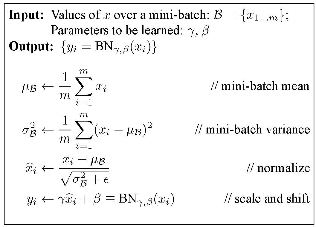
$\gamma$ and $\beta$ are important because it allows the network to recover any necessary mean-variance combination if the zero-mean / unit-variance isn’t optimal for the layer.

Difference with Layer Norm

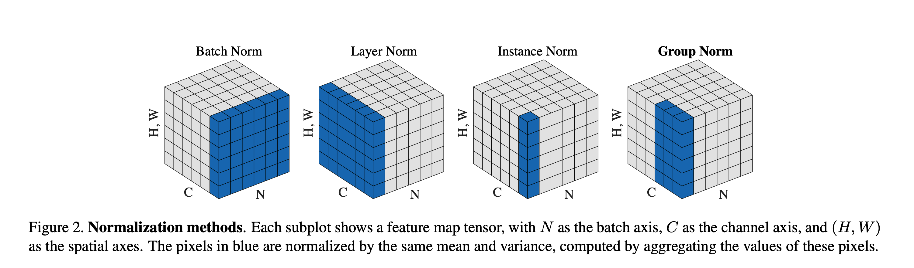
In a tensor of dimensions ($HW, N, C$) where

• $N$ (Batch Size) How many samples you’re processing in one pass.
• C (Channels) The “depth” of each activation map.
• H (Height) and W (Width) The spatial dimensions of each feature map.  For example a 224×224 image, H = 224 and W = 224 at input.

When we apply Batch Normalization to a convolutional layer, we are normalizing per-channel across all the data you have in that batch (N), that’s N samples × H × W values.

In contrast, Layer Normalization normalizes Across C × H × W For each sample independently, it treats all channels and spatial locations as one vector ($C × H × W$) and normalizes within that. That makes sense if you only ever see one example at a time (e.g. in [[Recurrent Neural Networks|RNN]]) or have tiny batches ($m< 4$)

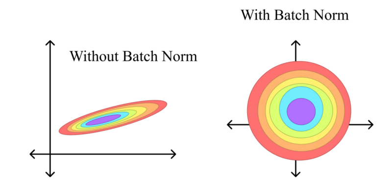
Speeds up training and less importance to initial weight

If we plot the loss in both approaches (No Normalization and Batch Norm) we can appreciate the improvements. On the left, without BatchNorm, the loss surface is shaped like a long, skinny ellipse: one direction is very steep, the other almost flat. If you pick a large learning rate, you’ll overshoot along the steep axis; if you pick a small one, we will be moving forward along the shallow axis. Training then becomes hard as we would have to just the right step size, and the weight initialization becomes more important as different weights can result in only a few hundreds steps until convergence or thousands.

On the contrary, once we insert BatchNorm between layers each hidden activation is recentered to zero mean and rescaled to unit variance (before stretching and shifting it again with $\gamma$ and $\beta$). This reshapes the loss into something much closer to a circle, where curvature is roughly the same in every direction. Now a single learning-rate setting makes balanced progress no matter which way we step. In practice this means we can have larger values for the learning rate and converge in far fewer epochs. Equally important, because BatchNorm is normalizing on the fly, the choice of initial weight scale matters less, even if starting with weights that would normally increase the number of epochs, the normalization layers help.