Neural Machine Translation By Jointly Learning to Align and Translate Explained

In order to understand attention, we will begin by revisiting the soft‐attention mechanism, one of the earliest and most influential forms of attention in neural sequence models. In “Neural Machine Translation by Jointly Learning to Align and Translate” (ICLR 2015), Bahdanau and colleagues observed that forcing an entire input sentence into a single fixed-length vector creates a bottleneck, especially for long or complex sequences. Rather than squash all information into one summary vector, their model produces a separate annotation vector for each source word and then, at each decoding step, computes a tailored context by softly selecting and combining just the relevant annotations. In this way, the decoder need only attend to the parts of the input that matter most for generating the next target word, allowing the system to capture rich, long-range dependencies without overwhelming a single fixed representation. We will cover all this into detail along with the architecture presented in the paper.

A normal encoder-decoder architecture would encode the whole input sequence into a fixed-length vector. Like so

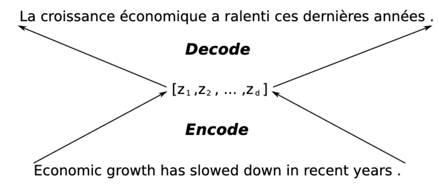
Instead, the proposed model encodes the input into a sequence of vectors and chooses only the relevant subset of vectors while decoding the translation (hence the title of the paper). This allows the model to deal better with long sentences because it doesn’t have to squash all the information into a fixed vector ($Z$)

The traditional approach: Encoder-Decoder with fixed sized vector $c$

In a normal RNN, the hidden state at time $t$ is created through a non-linear activation function ($f$) over the previous state ($h_{(t-1)}$) and the input at that time ($x_t$)

Here, $f$ can be a LSTM unit, $tanh(\cdot)$ etc.

In a “traditional” RNN Encoder-Decoder architecture the encoder would use these hidden states ($\overrightarrow h_i$) to create a fixed length vector $c$ by doing something like

Where $g$ is another non-linear function like $f$

We can draw the encoder architecture then to something like this:

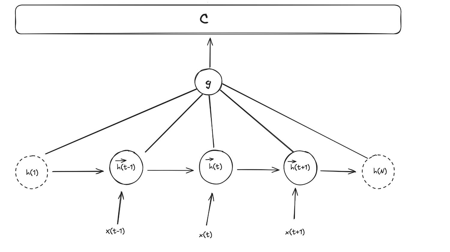
As we’ve said, creating a single length-fixed vector that squash all the information from the hidden states comes at the risk of losing some of the important information, specially in long sequences.

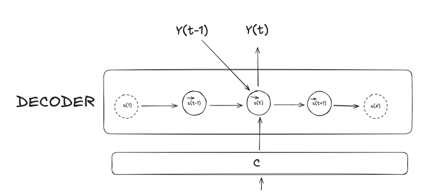
Then, the decoder architecture would use this vector $C$ as it is at each step $t$ where it would compute the conditional probability for word $y_t$ given also the previous hidden sate (let’s call it $s_{(t-1)}$), the previous word, $y_{(t-1)}$:

Again, $q$ is some sort of non-linear function that outputs the probability of $y_t$

Self-attention: variable vector $ci$

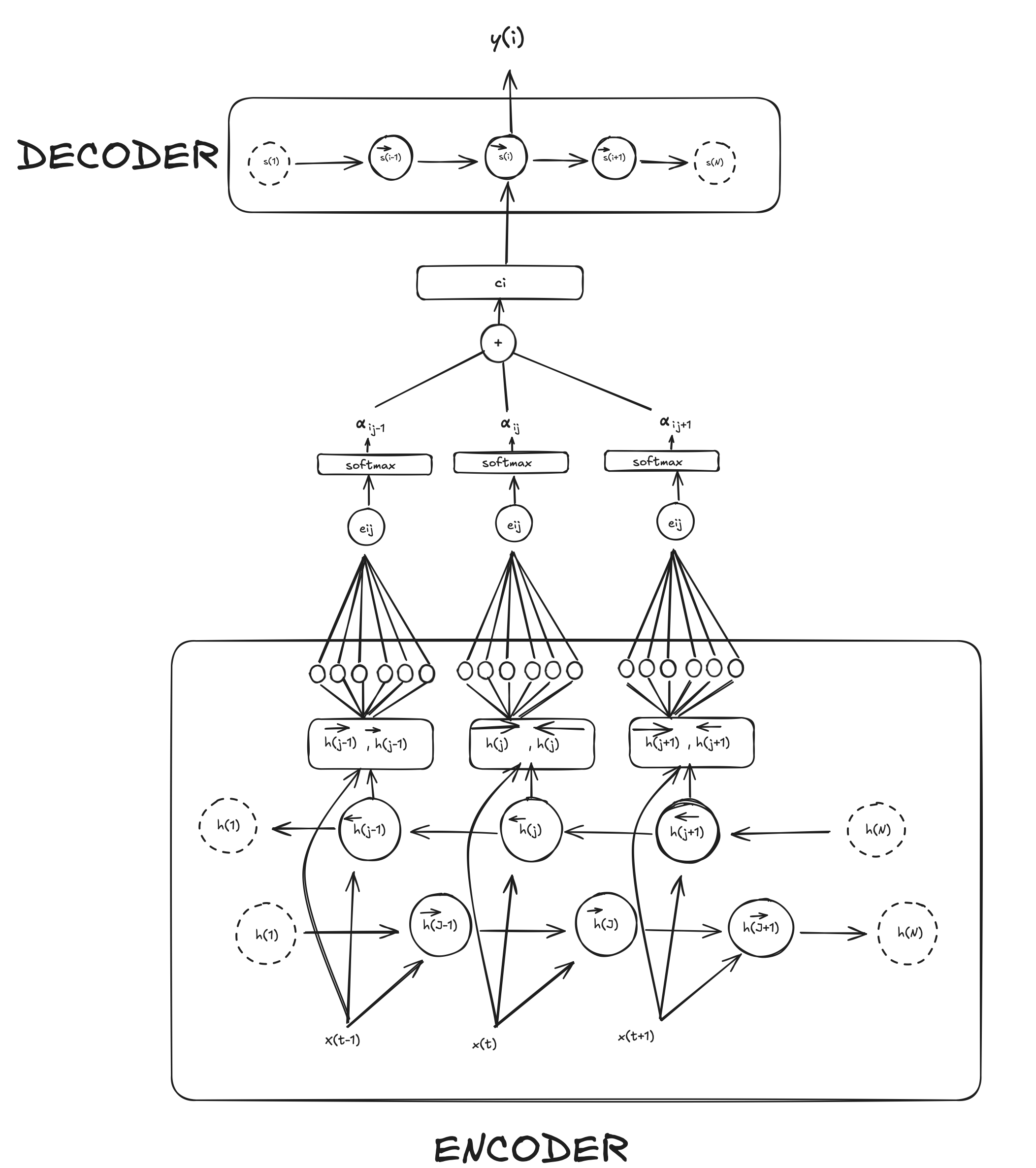
Instead of passing a single vector $C$ to the decoder, we are goin to create a variable vector ($c_i$) called the context vector which is computed as a weighted sum of annotations ($h_i$). This will make more sense as we see each part.

Encoder

The encoder consist of a Bidirectional Recurrent Neural Network (BiRNN). As the name suggest, a forward Recurrent neural network reads the input sequence ($[x_1, \dots x_N]$) from start to end ($1 \rightarrow N$) creating the hidden state ($\overrightarrow h_i$) while a backward RNN read the input sequence from end to start ($1 \leftarrow t$) creating the hidden state $\overleftarrow h_i$.

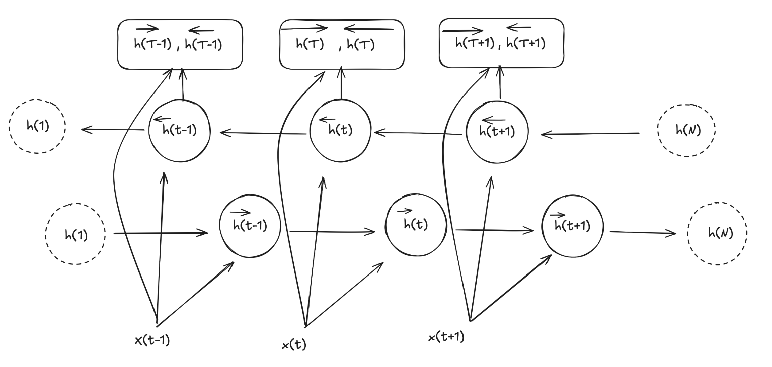
As in normal RNN, the hidden state at time $t$ is created through a non-linear activation function ($f$) over the previous state ($h_{(t-1)}$) and the input at that time ($x_t$)

Here, $f$ can be a LSTM unit, $tanh(\cdot)$ etc.

As I mentioned, the decoder is going to receive a variable context vector ($c_i$) that depends on annotations. These annotations ($h_j$) are created for each word ($x_j$) by concatenating the forward hidden state ($\overrightarrow h_j$) with the backward hidden state ($\overleftarrow h_j$) like so:

In this way, we can for each word an annotation that contains the summaries of both the preceding words and the following words.

Now, how is the context vector ($c_i$) created then? It is computed as a weight sum of these annotations

where $\alpha_{ij}$ is the weight for each annotation and is computed as

You may have realized that here we’re just applying a good-old softmax on $e_{ij}$ which stands for “energy” and reflects the importance that the annotation $h_j$ with respect to the previous decoder hidden state ($s_{i-1}$) in deciding the next state $s_i$ and generating $y_i$. Concretely, for each target position $i$ and each source annotation $h_j$ the model first computes an energy score $e_{ij}$ by feeding the pair ($s_{i-1}, h_j$) into a tiny feed-forward neural network $a$

 In practice this “alignment model” is a single hidden layer MLP: it linearly projects $s_{i−1}$ and $h_j$ via learned matrices $W_a$ and $U_a$, sums them, applies a $tanh$ nonlinearity, and then takes an inner product with a learned vector $v_a$ to produce the scalar $e_{ij}$. These parameters $W_a, U_a$ and $v_a$ are trained alongside all the encoder and decoder weights by back-propagating the translation loss through the softmax and through the MLP itself. So we can rewrite $e$ as:

To recap everything, we calculate a scalar $e_{ij}$ through an “alignment model” that linearly projects the previous hidden state in the decoder $s_{i−1}$ and the hidden state in the encoder $h_j$. Then we apply softmax to get the probability ($\alpha_{ij}$) for how, for a given word $i$, all the hidden states ($j$) impact with respect to the previous state ($s_{i-1}$). Then we create a context vector for that word ($c_i$) by calculating the weighted (through $\alpha$) sum of all hidden states $h_j$.

Roughly, this is what calculating $\alpha_{ij}$ looks like

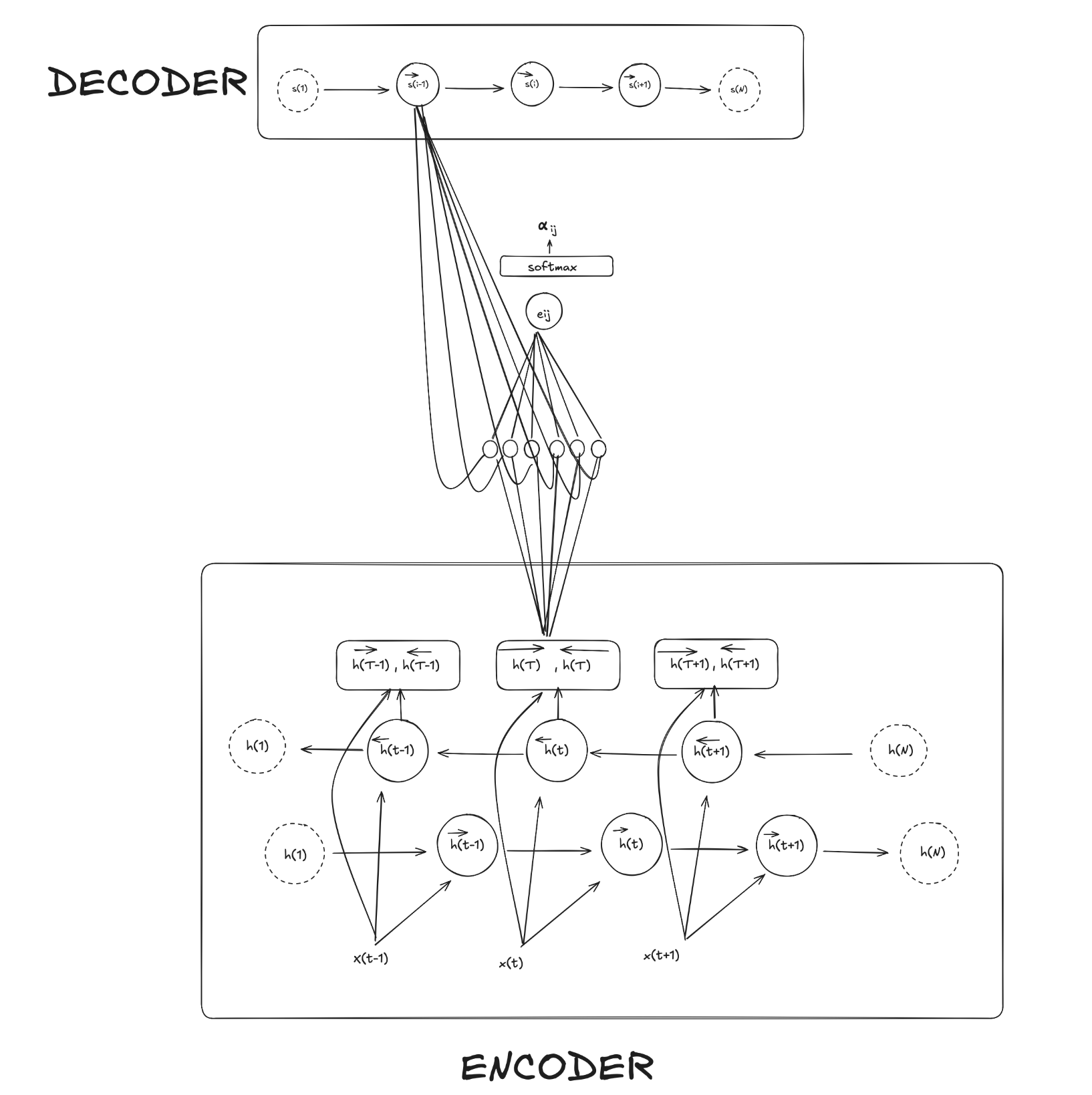
If we remove the lines from the hidden state in the decoder so its cleaner, this is how it looks like for all $\alpha_{i}$. To create the $c_i$ vector we just do the weighted sum.

Decoder

Finally, with the variable vector $c_i$, the previous hidden state $s_{(i-1)}$ and preceding words we can calculate each conditional probability in pretty much the same as the old decoder architecture. Only this time $c_i$ is a variable vector.

Similarly, each hidden state can be calculated as:

In the paper $f$ is a GRU (Gated Recurrent Unit).

Then, $s_i$ is combined with the context $c_i$, and often the embedding of the previous word $y_{i-1}$ into an intermediate vector, typically by concatenation followed by a linear layer and nonlinearity.  In the paper this is written as:

And then $\tilde s_i$ is projected into a $\lvert V\rvert$-dimensional vector of scores (one per target‐word in the vocabulary) and apply softmax:

The $j-th$ component of that softmax is the model’s predicted probability of emitting the $j-th$ word in the vocab at step $i$.  Selecting the highest-probability word gives the output $y_i$.

That’s pretty much it. Thanks for reading!