
Ridge Regression from Scratch
Published:
Recalling the classical linear‐least‐squares problem Given a dataset of $n$ observations and their correspondent responses $y_i$, we seek a parameter vector $\theta = (\theta_0,\dots,\theta_n)$ that minimizes the residual sum of squares (or the sum of squared estimate of errors):
\[J(\theta) \frac{1}{n} \sum_{i=1}^n \bigl(y^{(i)} - \theta^\top x^{(i)}\bigr)^2\]We would like to penalize large values of $\theta$, gently “pulling” the parameters toward zero. This discourages the model from relying overly on any single (possibly noisy) direction in feature space.
Let’s say we plot the ordinary least squares (OLS) cost function assuming only two parameters
 Image from https://allmodelsarewrong.github.io/ridge.html
The OLS solution would be the one that minimizes the Error surface (center of the sphere in 2D), introducing the regularization we try to pull the parameters from finding the OLS solution by imposing a small constrain. This allows the model to avoid overfitting
The second picture (the orange disk) shows the set of all $\theta=(\theta_1,\theta_2)$ such that
\[\theta_1^2 + \theta_2^2 \;\le\; c\]That is literally a circle (in 2D) of radius $\sqrt{c}$. Inside that circle, the length ($\mathcal{l}_2$‐norm) of the coefficient vector is at most $\sqrt{c}.$

Image from https://allmodelsarewrong.github.io/ridge.html
This in practice means that our $\theta$ can only take values that lies inside the $c$ circle. Were the circle big enough and we could find the exact same solution as in OLS.
The point of first contact is your Ridge solution: it’s the \theta with minimal error among all vectors of length at most $\sqrt{c}$
In practice, how do we impose said constrain in our model? We do it by using $\lambda$. We can think of it as a one to one correspondence with $c$.
{: .notice–info} $c$ and $\lambda$
- Small $c$ (or large $\lambda$) The orange circle is tiny. The best‐error ellipse that can touch it is still relatively large forcing $\theta$ very close to zero (strong shrinkage, high bias, low variance).
- Large $c$ (or small $\lambda$) The circle expands. We allow more complex $\theta$, so the optimal point moves out toward the unconstrained OLS solution (lower bias, higher variance)
Now our cost function with the added penalization term looks like this:
\[J(\theta) \frac{1}{n} \sum_{i=1}^n \bigl(y^{(i)} - \theta^\top x^{(i)}\bigr)^2 + \lambda \sum^p_{j=1} (\theta_j^2)\]When computing the gradient w.r.t. $W$ we end up with:
\[\nabla J(\theta) = \frac{2}{n}\;X^\top\,(X\theta - y) \;+\; 2\,\lambda\,\theta\]See how in the cost is written as \(\tfrac1n\sum_i (y^{(i)} - \theta^\top x^{(i)})^2\) but the gradient ends up involving to \(\theta^\top x^{(i)} - y^{(i)}\) That is because When you take the derivative of the square $(y - f)^2$, the “inside” $y - f$ produces a minus sign, which flips the order:
\[\frac{d}{df}\bigl(y - f\bigr)^2 =2\,(y - f)\,\frac{d}{df}(y - f) =-2\,(y - f) =2\,(f - y)\]We can update our parameter in gradient-descent as:
\[\theta \;\gets\;\theta \;-\;\eta\;\Bigl[\tfrac{2}{n}X^\top(X\theta - y) \;+\;2\lambda\,\theta\Bigr]\]In python this would be:
w_grad = (2 / X_train.shape[0])* X_train.T.dot(error) + 2*self.reg_factor*(self.W.T)
self.W -= self.lr * w_grad
The rest of the model is implemented as a normal Linear Regression
How to chose $\lambda$?
In practice, $\lambda$ is a parameter we can only chose through testing. As we’ve seen we have a tradeoff between a small $\lambda$ which implies getting closer to the OLS solution (low bias, high variance if overfitted) or large $\lambda$ where we shrink the coefficients towards zero (higher bias, low variance).
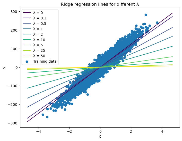
If we plot how this factor changes our prediction model we see that as $\lambda$ increases the slope approximates zero and moves away from the OLS solution (i.e. $\lambda = 0$)
Comments