LSH Forest

Locality-sensitive hashing or LSH, allows us to focus on pairs that are likely to be similar, instead of having to look at all pairs possible. It reduces therefore the amount of computational time required by a brute force approach.

In essence, we take the items, we obtain a hash of these items and store them in buckets with other items with similar hashes. What we are trying to accomplish is to aggregate into a bucket those items with similar hashes to then only search for similar pairs within the bucket instead of looking at all possibilities. This of course requires that similar items will have similar hashes. That is why the hash functions we’re using are carefully designed.

There are 3 fundamental steps in this process:

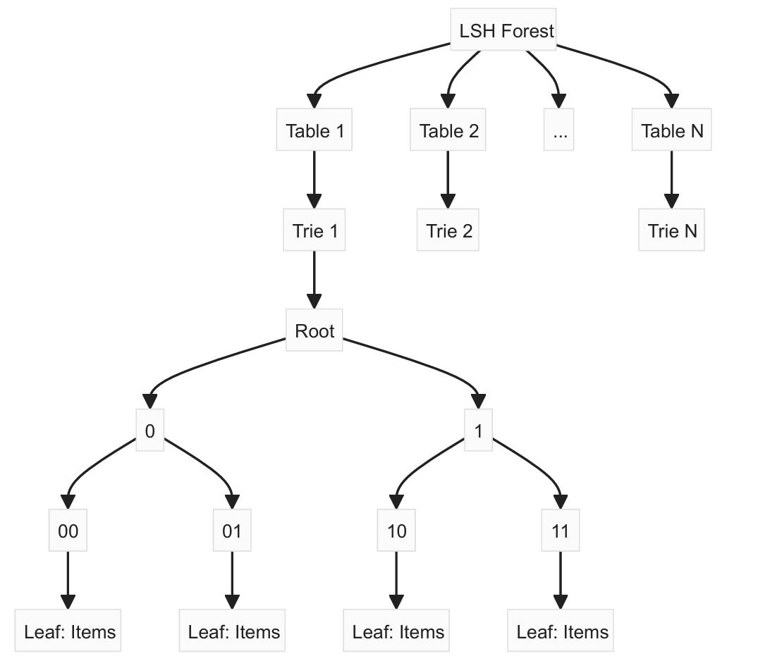
1. Creating multiple LSH tables, each using a subset of the MinHash signature
2. Each table is structured as a prefix tree (trie) for quick lookup
3. When querying, traverse the trees to find candidate nearest neighbours.

What is a LSH Table?

A LSH table is a data structure that groups similar items together based on their hash values. Each item -molecules in our case- has its own MinHash vecotr, and all of these vectors are stored in the LSH Table.

Let’s do a practical example:

Creating multiple LSH tables, each using a subset of the MinHash signature

1. Original Fingerprint Let’s say we have a 16-bit fingerprint for a molecule: 1011000110101101

2. MinHash Transformation We apply multiple hash functions to this fingerprint. For simplicity, let’s say we use 4 hash functions, resulting in a MinHash signature of 4 integers: [42, 17, 93, 28]

To remember how this MinHash signature is calculated see the example on the MinHash blogpost

1. LSH Table Creation Let’s assume we’re creating 2 LSH Tables, each using 2 of the 4 MinHash values (a subset of the MinHash)

• Table 1 uses [42, 17]
• Table 2 uses [93, 28]

We’ll focus on Table 1 for this example.

1. Binary Representation We convert the MinHash values to binary. Let’s say we’re using the last 4 bits of each number: 42 -> 101010 -> 1010 17 -> 010001 -> 0001

So for Table 1, our hash becomes: 10100001

Each table is structured as a prefix tree (trie) for quick lookup

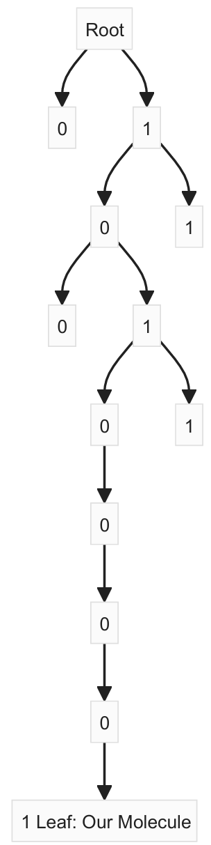
1. Trie construction We insert this binary string into the trie. Each bit determines which path to take at each level.

1. Searching for Similar Items: When searching for ismilar items, we follow the same process.
   1. Generate fingerprint for our molecule
   2. Create its MinHash signature
   3. Use the subset for Table 1 (in this case, the first 2 MinHash values)
   4. Convert to binary
   5. Traverse the trie

Once we reach a leaf node, all the items stored at this leaf and nearby leaves are considered candidate nearest neighbours.

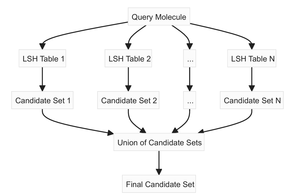
When querying, traverse the trees to find candidate nearest neighbours.

Since we have several LSH tables, the algorithm actually uses all the LSH tables simultaneously, rather than selecting a single table. This improves the accuracy of the approximate nearest neighbour search. From each table, the algorithm collects a set of candidate nearest neighbours. The final set of candidate nearest neighbors is the union of candidates from all tables.

Bibliography:

• Mining of Massive Datasets - Jure Leskovec, Anand Rajaraman & Jeffrey D. Ullman